Adding Boundary Geometries
The data that the scientists want to ingest is summarized in the CDC Zika Repository. If you open up the data for Argentina, you’ll notice that the data looks pretty similiar to last mission, except that there is no latitude or longitude to geocode each row; however, each row does have a location field. We should be able to indentify those locations to actual areas on a map.
Search for “political boundaries geojson” and find gadm.org. This site provides geospatial data about administrative boundaries for each state. Go to the GADM Downloads Page to check out the data.
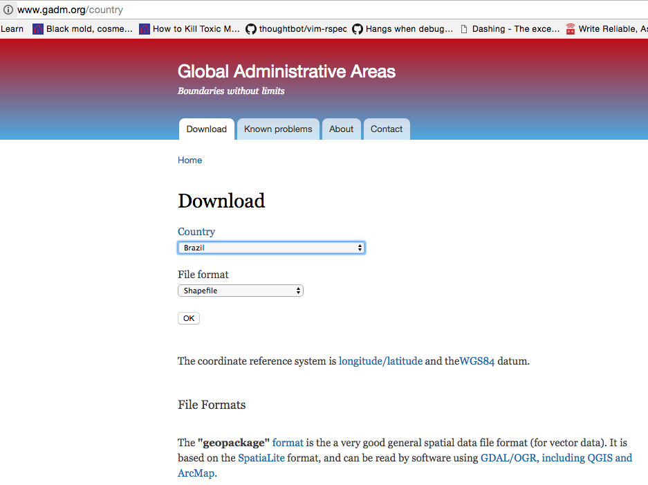
Download the shapefile for Brazil.
The file BRA_adm_shp.zip will download. Double click the file to unzip the file. You should see three shapefiles: BRA_adm0.shp, BRA_adm1.shp, BRA_adm2.shp. BRA_adm3.shp. Let’s take a look at these shapefiles. In order to look at a shapefile, you will need download QGIS, an open source desktop viewer for geospatial data. QGIS can be downloaded via the Boundless site. After downloading, double click the .dmg file to install.
Note
Note: Use your personal email to register on Boundless Connect to get access to the QGIS download.
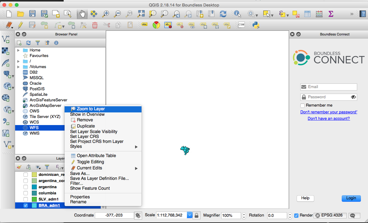
After QGIS is installed, drag the BRA_adm1.shp file into the QGIS window in order to import the file.
Note
The zoom on the QGIS window is VERY sensitive. You may need to automatically zoom to the layer you would like to view. Right click on your layer in the Layers Panel, and select Zoom to Layer.
Great! That looks exactly like what we need. Let’s convert the file into GeoJSON so that we can serve it up from within our web application. We can use the ogr2ogr command.
$ ogr2ogr -f "GeoJSON" brazil.geojson BRA_adm_shp/BRA_adm1.shp
After the command completes, check out the brazil.geojson file. Yikes! The file seems pretty big. Let’s see how big:
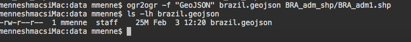
A 25M file is not going to work well in our web app. And that’s just Brazil!
Fortunately, shapefiles can be compressed in size by reducing the amount of detail. In QGIS, select Vector > Geometry Tools > Simplify geometries from the top menu. Select your Brazil Geometry BRA_adm1 and set the tolerance to 0.05. Hit Run.
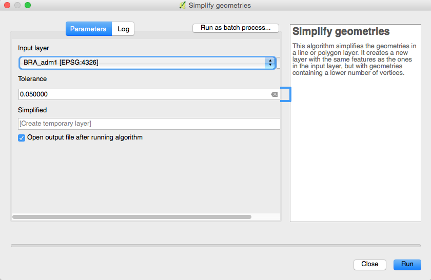
QGIS should generate a new layer that looks pretty much the same as the last layer.
Right click on the newly created layer and select Save As…. Save the file as GeoJSON with the name brazil_compressed.geojson. Be sure to type in the entire path of the file that you are creating.
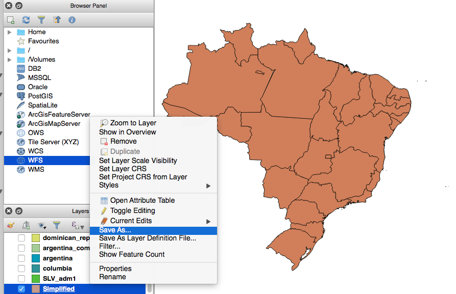
Now if you check the size of the newly created brazil_compressed.geojson, you should see that it is much smaller!
Run the command:
$ ls -lh brazil_compressed.geojson

Note
A file size of 331K isn’t great for a webapp; it’s still a bit large. In a few weeks, we’ll look at how some of the features of GeoServer allows you to display large amounts of data without a big download.
The last step is to join all of the GeoJSON files together. To do that, we can use a nice Node.js library from MapBox. Run the following commands:
$ npm install -g @mapbox/geojson-merge
$ geojson-merge argentina_compressed.geojson brazil_compressed.geojson columbia_compressed.geojson dominican_republic_compressed.geojson el_salvador_compressed.geojson equador_compressed.geojson guatamala_compressed.geojson haiti_compressed.geojson mexico_compressed.geojson
nicaragua_compressed.geojson panama_compressed.geojson > states.geojson
To save you time, we went ahead and optimized the geometries for each country. Some might still need some work, but can
tackle that some day when you are bored.